• Approximating Digital Functions
• Iteration
• Sums
• Products
• A Quadratic Product
• Recursive Types and Recursion
• Quicksort, First Pass
• Defunctionalization
• Final Quicksort
• Final Thoughts

Introduction

I’ve been a bit obsessed with continuous computation recently. Both in the sense of analog computing and the sense of coinduction. I want to write a post about the latter eventually, but this post will be focused on analog computation. Specifically, how one might compute digital functions inside a continuous domain. By the end of this post I want to have a function S : ℝ → ℝ whose action is, in some sense, equivalent to that of Quicksort, since that seems like a well-known enough discrete algorithm which also requires all the techniques I want to talk about.

This post is a follow-up to my last post on bijective encodings, so you may want to read that first if you haven’t.

The ultimate inspiration for this post is this article;

• Robust Simulations of Turing Machines with Analytic Maps and Flows by Daniel S. Graća, Manuel L. Campagnolo, and Jorge Buescu

The overall concept of that paper is to define, given a Turing machine, an ODE whose action corresponds to the evaluation of said machine. Much of the paper pertains to particular, somewhat tedious, numerical functions for various specifics, but the general concept is quite straightforward. They start by encoding the transition of the Turing machine as a function ℕ³ → ℕ³, where the three natural numbers encode, respectively, the state, the tape left of the head, and the tape right of the head. They then construct an analytic function ℝ³ → ℝ³ with an error term which, as the error approaches 0, approaches the discrete function on natural inputs. This is then used to create a function ℝ⁴ → ℝ³, where the extra real is a variable, t, for time, representing the number of times the transition function is iterated. If the function halts, then there exists a well-defined limit as t approaches infinity defining the output state of the machine on a given input. Ultimately everything is described in terms of solutions to polynomial ODEs, showing that they are Turing complete.

I won’t go into the specifics of the paper beyond that. In some sense, I could end the post there since we can select a universal Turing machine and implement whatever algorithm we want on that machine, and shove it into the equation described in that paper. But that’s not very enlightening, and it’s even less useful. Instead, I want to take the encodings of the many discrete types described in my last post and use similar techniques to make them continuous. The exercise was, at least to me, somewhat eye-opening and really puts into focus the relation between analog and digital computation.

Approximating Digital Functions

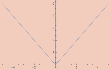
Anyone who’s done anything with digital circuitry probably won’t be too surprised at where we start. I need a library of discrete signals which can be effectively approximated by a continuous analytic function. This means square waves, triangle waves, sawtooth waves, floor functions, absolute value functions, step functions, and probably other things that I won’t need but which might be needed for other particular purposes. None of these functions are smooth and most aren’t continuous. As a consequence, they can’t be derived on the nose by analog methods, but we can define analog functions with an error term that we can control.

These constructions are significant as it pertains to real computability. The original notion of real computability as described by Shannon excludes many basic (Abs) and not so basic (Gamma) functions from being computed. Essentially, computability in his sense required the existence of an ODE whose solution at t=1 coincides exactly with whatever function we’re computing. Contrast this with coinductive/type-2 approaches to real computability where we never have all the data of a function instantaneously and only require the ability to compute more and more exact values with more effort. More recent work changes this definition of computability to allow asymptotically approximating a function using an error term. There are a couple of different variations of “real recursive calculi”; variations of μ-recursive calculi which use real numbers instead of natural numbers. Such systems sometimes allow infinite limits to be taken, acting as the continuous analog of the μ-operator/minimization/while-loop. Much like the μ-operator, the limit’s return value is not, in general, well-defined. With that change, the real functions definable in the presence of a noise floor are exactly the computable functions in the coinductive/type-2 sense.

• A Foundation for Real Recursive Function Theory by José Félix Costa, Bruno Loff, and Jerzy Myckac

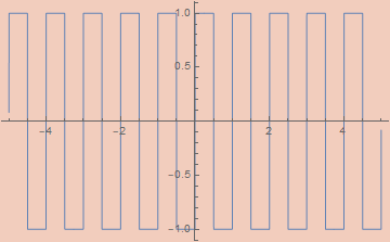
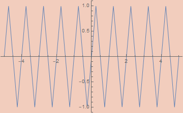
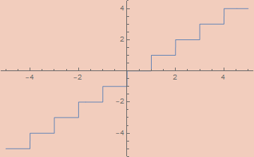
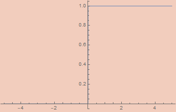
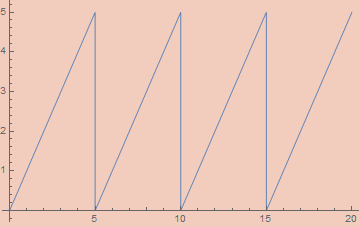
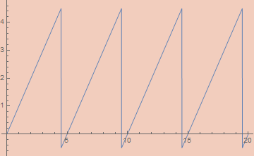
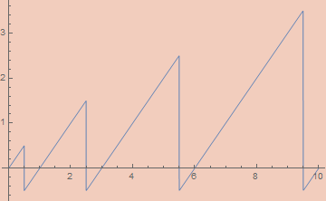
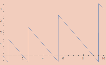
I don’t have much interesting to say about the functions themselves, so I’ll just list them and their definitions. For each, the error, ε, has been set to 10^-5 in the graphs.

εAbs[ε_, x_] := x Tanh[x/ε]

εSquareWave[ε_, x_] := (2/π) ArcCot[ε Csc[2 π x]]

εTriangleWave[ε_, x_] := (2/π) ArcSin[(1 - ε) Cos[2 π x]]

εSawtoothWave[ε_, x_] := 
  (εTriangleWave[ε, x/2] εSquareWave[ε, -x/2] + 1)/2

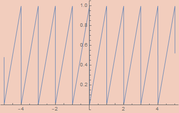
Note: A reasonable looking definition for εSawtoothWave is 1/2 - ArcTan[(1 - ε) Cot[π x]]/π, but this doesn’t work since Cot is undefined on numerous arguments.

εFloor[ε_, x_] := x - εSawtoothWave[ε, x]

Round[x_] := Floor[x + 1/2]
Ceiling[x_] := Floor[x + 1]

εUnitStep[ε_, x_] := ArcTan[x/ε]/π + 1/2

Iteration

One of the most basic discrete activities is that of iteration; taking a function f and applying it a fixed number of times to define a new function. Defining iteration in a continuous way is the key that unlocks universal computation, so I think it’s worth going through upfront.

There is no common function which implements what we want; instead, we need to set up a simple ODE whose solution is (asymptotically) a step function that takes a step the size of f each unit.

The basic idea is simple. We’ll end up making an analog, uh, analog of a latch. We’ll have two variables, x and y, with x being our step function. At each time interval of unit length, we’ll apply f to y and store it in x while also copying the value of y into x for the next iteration. To do this using differential equations, we’ll do the first task between t and t + 1/2 and the second task between t + 1/2 and t + 1. To accomplish this, we want x to be constant on [t, t + 1/2] while y is constant on [t + 1/2, t + 1]. This requires the derivatives to be 0 within their respective intervals. At the same time, we want the derivative of y to be 2 (f[x] - x) on [t, t + 1/2] so that its value reaches f[x] within a half unit of time. This means using a square wave to mask out the respective intervals. Note that y and x should have the same value at the end of each unit interval. We also want the derivative of x to be (2 (y - x))/SawtoothWave[2 t] on [t + 1/2, t + 1] for similar reasons. This derivative will wipe out the entire value of x in half an interval while replacing it with the value y. The net consequence of this system will be a continuous functional solution to y and x which simulates the iteration of f.

Putting all these ideas together, we end up with the following system of first-order differential equations.

x'[t] == (2 (y[t] - x[t]))/εSawtoothWave[ε, 2 t] * (εSquareWave[ε, t + 1/2] + 1)/2
y'[t] == 2 (f[x[t]] - x[t]) (εSquareWave[ε, t] + 1)/2
x[0] == x0, y[0] == x0

And shoving this inside of NDSolve on a few test inputs gets us the following graphs, where orange is x, blue is y, and the green dots are the results of actual iteration.

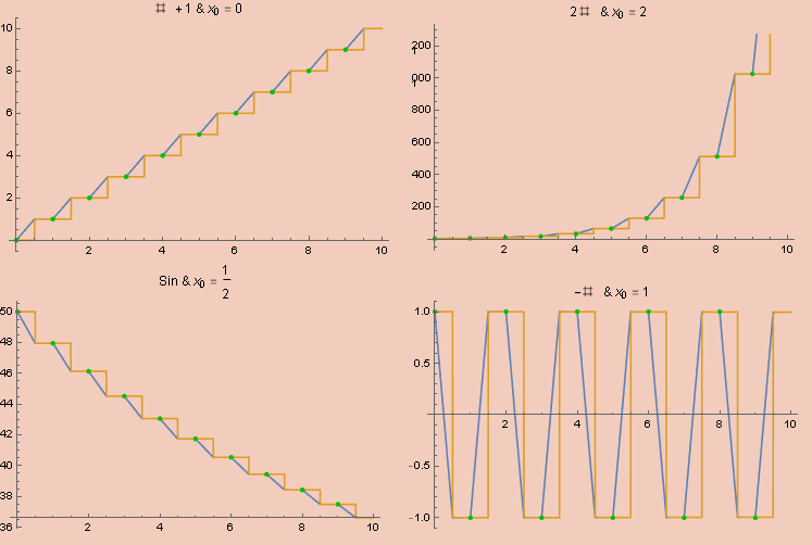
While we don’t get an expression in terms of elementary functions, this is perfectly well-defined as an analog computation. For quicker experimentation, we can define the function x limits to as;

cIterate[f_, x0_][n_] := Nest[f, x0, Round@n]

Sums

Stepping back to the encodings from my last post, something I want to emphasize is that we’re sticking exclusively to numbers. For the purposes of this post, trees will be numbers, lists will be numbers, lambda expressions will be numbers, etc. We aren’t going to be encoding/decoding into some nice-looking syntax. This has some important consequences. Mainly, we’ll be focusing on the functions needed to manipulate already encoded data. The functions I’ll be defining are the standard combinators emerging from the universal properties of the types in question. The same ones are used in the algebra of programming. See

• Program Design by Calculation by J. N. Oliveira

Since our encodings are bijective, any data can be interpreted as being of any type isomorphic to ℕ. So a function like n² : ℕ → ℕ can be interpreted instead as a function from lists to trees, or lambda expressions to sorted lists, or formulas of some theory to rational numbers, etc. It’s not always useful to think in this way, but you’ll never get something that’s truly nonsensical as all data will encode a valid, and unique, term of any countable type. So, whenever you see me mention ℕ in this post, you can replace it with any countable type in your head, if you want.

In my last post, I started with encoding tuples and sums. Sums are the easier case, so I’ll start with them.

There are two classes of functions we need for sums; constructors and destructors.

In the simple case of ℕ + ℕ, the constructors are often denoted inl and inr or Left and Right, etc. In general, we can interpret a sum ℕ + ℕ + ℕ + … + ℕ as n × ℕ, the product of a finite type of size n with ℕ. We can then describe constructors as pairs, (k, m) where k < n and m ∈ ℕ. We also have the case of summing ℕ with a finite set, n + ℕ. Since any repeated finite sets sums, n + m + … + ℕ can be rolled into a single finite set (n + m + …) + ℕ, we only need to address the binary case for full coverage.

Starting with the ℕ + ℕ case, the constructors just add a bit to the number, either 0 or 1 depending on the constructor, so that’s easy to implement.

inl[x_] := 2 * x
inr[x_] := 2 * x + 1

Generalizing to the n × ℕ case is a minor variation of these functions.

in[n_, k_][x_] /; k < n := n * x + k

In the case of n + ℕ, we bijectively encode these elements by interpreting all numbers i < n as i (in other words, we do nothing to them) and interpreting all numbers i ≥ n as i-n. The constructors are then very simple.

finInl[n_][k_] /; k < n := k
finInr[n_][k_] := k + n

To make the destructors, we need to be able to strip off the constructor to get the data being tagged in the first place. This stripping function is called the “codiagonal”. In the ℕ + ℕ case, this simply strips off the least significant bit. We can accomplish this by dividing by 2 and flooring.

Codiagonal[x_] := Floor[x/2]

We can generalize beyond binary coproducts fairly easily by stripping off the least significant nit from data of type n × ℕ.

NCodiagonal[n_][x_] := Floor[x/n]

This is, incidentally, the same thing as the second projection out of the finite product; n × ℕ → ℕ.

The actual constructor, the k in (k, m) ∈ n × ℕ, can be recovered using a simple mod.

NProj[n_][x_] := Mod[x, n]

In the n + ℕ case, we can implement the codiagonal like so;

FinCodiagonal[n_][x_] /; x < n := x
FinCodiagonal[n_][x_] := x - n

To take this to the continuous setting, we can use the step function to decide if we should subtract n.

FinCodiagonal[n_][x_] := x - n UnitStep[x - n]

The destructors for sums are characterized by fusion functions. These will have a list of functions, one for each possible entry in a sum. The fusion function figures out which entry in the sum we have and applies the appropriate function. If we have an entry (k, m) ∈ n × ℕ and a list of n functions, fns, fuse(fns, (k, m)) will return fns[[k]](m), the kth function applied to m.

In the ℕ + ℕ case, the fuse function will, given two functions f and g, apply f in the inl case and g in the inr case. We need a function for detecting the constructor. This is done through modding. As it turns out, modding is a minor variation of the sawtooth function.

εMod2[ε_, x_] := 2 εSawtoothWave[ε, x/2]

Of course, this doesn’t quite work in general, as one can’t reliably ascertain the value when the result should be 0. To do this, we merely perturb the input and output by 1/2. We can generalize to arbitrary mods pretty easily;

preεMod[ε_, x_, n_] := n εSawtoothWave[ε, x/n]
εMod[ε_, x_, n_] := preεMod[ε, x + 1/2, n] - 1/2

Using this, we can implement an if statement. Mod[x + 1, 2] a + Mod[x, 2] b will be a when x is even and b when x is odd. We can use this trick to implement fuse.

Fuse[f_, g_][x_] := Mod[x + 1, 2] f[Codiagonal[x]] + Mod[x, 2] g[Codiagonal[x]]

We can further generalize to arbitrary n, given a list of functions.

NFuse[fns_][n_] :=
  With[{l = Length@fns},
    Sum[Mod[n + i, l]*fns[[i]][NCodiagonal[n][l]], {i, 1, l}]
  ]

Fusion in the n + ℕ case requires a similar decision procedure.

FinFuse[n_, f_, g_][x_] /; x < n := f[x]
FinFuse[n_, f_, g_][x_] /; x >= n := g[x - n]

We need a method to check for the relative size of the input. We can use UnitStep to detect the negativity of n - k which will indicate if k is greater than n.

FinFuse[n_, f_, g_][x_] :=
  UnitStep[x - n + 1/2] g[x-n] + (1 - UnitStep[x - n + 1/2]) f[x]

We can now perform all standard manipulations on sums. One of the more helpful utility functions is the sum bimap which leaves the leading constructor of the sum intact while applying either f or g.

SumBimap[f_, g_] := Fuse[inl@*f, inr@*g]

In the n + ℕ case, we can use the appropriate fusion function as well.

FinSumMap[n_, f_] := FinFuse[n, # &, (n + #) &@*f]

In the n × ℕ case, we can do the following to map onto the second argument.

FinProdMap[n_, f_][x_] := in[n, NProj[n][x]][f[NCodiagonal[n][x]]]

Products

In my last post, I defined encodings of products ℕ × ℕ × … × ℕ for arbitrary many ℕs. This is unnecessary in theory as we can define them as ℕ × (ℕ × (ℕ × …)). There are lots and lots of encodings for products.

• The Rosenberg-Strong Pairing Function by Matthew P. Szudzik

In my last post, I used one based on bit interlacing, but this is hard to make continuous. I’ll start with use two encodings, the O.G. Cantor pairing and Sierpinski pairing. The pairing functions themselves are already analytic.

CantorPair[x_, y_] := (x^2 + 2 x y + y^2 + 3 x + y)/2

SierpinskiPair[x_, y_] := 2^x (2 y + 1) - 1

The reason I highlighted these is their packing characteristics. CantorPair packs things fairly, so a random number decoded into a Cantor pair will, on average, have both entries be about the same size. SierpinskiPair, on the other hand, packs y much more tightly than x so that a random number will decode to a pair where y is exponentially larger than x, on average. Depending on the application, both functions may have their uses.

The destructors for products are just the projection functions that extract the first and second elements. The universal constructor is a fork map that takes an argument, x, and two functions, f and g, and returns a pair (f[x], g[x]).

For cantor pairing, extracting the arguments seems at first to be fairly easy, requiring using the floor function. A standard definition is the following;

preFst[z_] := z - (#^2 + #)/2 &[Floor[(Sqrt[8 z + 1] - 1)/2]]
preSnd[z_] := (3 # + #^2)/2 - z &[Floor[(Sqrt[8 z + 1] - 1)/2]]

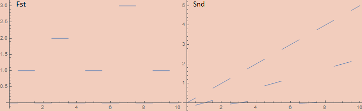
However, this doesn’t approach a correct Fst function as the error goes to zero. As a specific example, this Fst approaches 5/8 on the input 1 when it should approach 0 since CantorPair[0, 1] == 1. Since the slope of Fst is 1 and that of Snd is -1 on all inputs in the limit, we can do a similar trick we already did with Mod and perturb the input and output by 1/2. In the case of Fst, they’ll cancel out if their signs are opposite while they’ll cancel out with the same sign in Snd.

CantorFst[z_] := preFst[z + 1/2] - 1/2
CantorSnd[z_] := preSnd[z + 1/2] + 1/2

Projecting out of SierpinskiPair is more complicated. Standard implementations of projection functions require inspecting the binary expansion of the numbers. Specifically, the number of 1s at the end of the binary expansion of the number is the first number while the remaining bits (ignoring the last 0) encodes the second number. For example SierpinskiPair[7, 2345] == 600447 whose binary expansion is

10010010100101111111

There are 7 1s at the end, so that’s our first number. The remaining bits (ignoring the last 0) are 100100101001, which is the binary representation of 2345; our second entry.

These algorithms are not hard to implement. In fact, one of the projections is even a built-in function in Mathematica.

SierpinskiFst[z_] := IntegerExponent[z + 1, 2]
SierpinskiSnd[z_] := ((z + 1) 2^-SierpinskiFst[z] - 1)/2

However, these functions are tricky to make continuous. If the first can be made that way, the second comes along for free. The Fst function is simply the largest power of 2, n, such that Mod[z + 1, 2^n] == 0. This is the same as the number of powers of 2 greater than 0 which z is divisible by. We can actually calculate this by integration. Consider the graph of 1 - UnitStep[Mod[k, 2^Floor@n]-1/2]. At each unit interval, if the mod power of 2 is 0, the value will be 1 over that interval; if the mod power of 2 is greater than 0, the interval will be 0. By integrating that function from 1 to Ceiling[Log[2, z]], we’ll calculate the first component, adding 1 for every power of 2 which the number is divisible by.

SierpinskiFst[x_] :=
  Integrate[
    1 - UnitStep[Mod[x + 1, 2^Floor[n]] - 1/2],
    {n, 1, Ceiling[Log[2, x + 1]]}
  ]

Note that this implementation doesn’t really work. This is more of a design for a hypothetical analog circuit. If you want to play around with a continuous version of this function, use this, which isn’t really the same function, but it should work fine;

SierpinskiFst[z_] := IntegerExponent[Round[z] + 1, 2]

That basic trick of integrating something sandwiched between a step function and a floor function is a generic method for counting numbers satisfying some property in a continuous way. It’s a method for defining discrete sums in terms of continuous ones. Based on that, we can get the following alternative definition;

SierpinskiFst[x_] :=
  Sum[
    1 - UnitStep[Mod[x + 1, 2^n] - 1/2],
    {n, 1, Ceiling[Log[2, x + 1]]}
  ]

At this point, we can define the universal properties of the product fairly easily. The fork functions can be defined as;

CantorFork[f_, g_][x_] := CantorPair[f[x], g[x]]

SierpinskiFork[f_, g_][x_] := SierpinskiPair[f[x], g[x]]

and we can similarly define the product functorial bimap.

CantorBimap[f_, g_] := CantorFork[f @* CantorFst, g @* CantorSnd]

SierpinskiBimap[f_, g_] := SierpinskiFork[f @* SierpinskiFst, g @* SierpinskiSnd]

As a nice utility function, we can also define an uncurrying function that feeds a pair of values into a binary function.

CantorUncurry[f_][x_] := f[CantorFst@x, CantorSnd@x]

SierpinskiUncurry[f_][x_] := f[SierpinskiFst@x, SierpinskiSnd@x]

A Quadratic Product

I want to create a custom pairing function with a packing efficiency between Cantor and Sierpinski. Cantor packs x the same as y; Sierpinski packs y exponentially denser than x; what if we need something that packs one element merely quadratically denser?

This topic is explored in detail in the paper;

• Efficient Pairing Functions - and Why You Should Care by A. Rosenberg

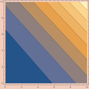
The paper outlines a procedure for creating Cantor-like pairing functions. This excludes something like the bit-manipulation pairing function I presented in my last post, but it offers a lot of flexibility and conceptual clarity. At its core, Cantor-like pairing functions define a series of shells which in total cover the integer parts of the positive plane. In the case of Cantor pairing itself, the shells are made up of relations of the form x + y = s, where s is the shell that contains the point (x, y). Have a look at the paper for some nice illustrations of these shells.

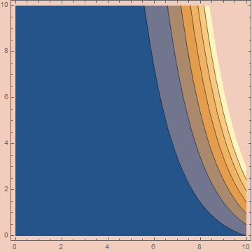
To pack a point quadratically tighter we can use shells of the form x² + y = s. This will create shells of the following shape;

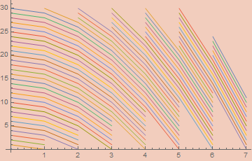
Each one of those lines corresponds to the curve s - x².

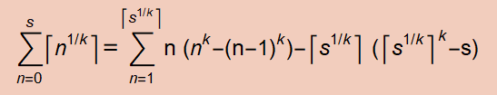
To actually define this pairing function, we need to identify the shell, the number of elements that preceded that shell, and how far along in the shell we are. Our shell is just x² + y. We may notice that shell s has Ceiling[Sqrt[s]] items in it. So summing that up to our shell and adding x (which tells us how far along the shell we are) gets us our encoding.

QuadPair[x_, y_] := Sum[Ceiling[Sqrt[n]], {n, 0, x^2 + y}] + x

This is all well and good, but it’s horrendously inefficient to actually carry out this sum. We may notice that

Sum[Ceiling[Sqrt[n]], {n, 0, s}]

is adding up (1² - 0²) 1s, (2² - 1²) 2s, (3² - 2²) 3s, etc. Based on that, we can get something close via;

Sum[n*(n^2 - (n - 1)^2), {n, 1, Ceiling[Sqrt[s]]}]

The error of this term is of order Ceiling[Sqrt[s]] and is proportional to the difference between Ceiling[Sqrt[s]]^2 and s. So, with some additional sum algebra, we can observe that

Sum[Ceiling[Sqrt[n]], {n, 0, s}]
== Sum[n*(n^2 - (n - 1)^2), {n, 1, Ceiling[Sqrt[s]]}]
   - Ceiling[Sqrt[s]]*(Ceiling[Sqrt[s]]^2 - s)
== (-(1/6) + s) Ceiling[Sqrt[s]] + 1/2 Ceiling[Sqrt[s]]^2 - 1/3 Ceiling[Sqrt[s]]^3
== (s - 1/6) # + 1/2 #^2 - 1/3 #^3 &[Ceiling[Sqrt[s]]]

allowing us to rewrite the pairing function as

CeilingSqrtSum[s_] := (s - 1/6) # + 1/2 #^2 - 1/3 #^3 &[Ceiling[Sqrt[s]]]
QuadPair[x_, y_] := CeilingSqrtSum[x^2 + y] + x

which is clearly efficient to evaluate. Of course, a pairing function isn’t so useful if it can’t be unpaired. The unpairing functions are conceptually simple. There’s a straightforward, if not so efficient, method for finding the shell of an encoded pair by simply finding the largest shell whose CeilingSqrtSum is below the input.

QuadShell[n_] :=
 Block[{s},
  s = 0;
  While[n - CeilingSqrtSum[s] ≥ 0, s++];
  s - 1]

With the shell in hand, the exact coordinates of an encoded pair, n, can be easily calculated.

QuadUnpair[n_] :=
  Block[{s, x, y},
    s = QuadShell@n;
    x = n - CeilingSqrtSum@s;
    y = s - x^2;
    {x, y}]
QuadFst[n_] := QuadUnpair[n][[1]]
QuadSnd[n_] := QuadUnpair[n][[2]]

However, that QuadShell implementation is clearly too slow for our purposes. There is an easy way to make it faster. We can remove the ceiling function from the CeilingSqrtSum function and calculate its inverse as the root of a particular polynomial. Taking the floor of that yields;

PreQuadShell[n_] := Floor@Root[-36 n^2 + (1 + 36 n) # - 17 #^2 + 16 #^3 &, 1]

Which is quite nice, I think, but is subject to periodic overestimations. We can use this as a first pass estimate and adjust accordingly;

QuadShell[n_] :=
 Block[{s},
   s = PreQuadShell[n];
   While[n - CeilingSqrtSum[s] < 0, s--];
   s
 ]

We can then get the same structural functions we had for the other pairing functions;

QuadFork[f_, g_][x_] := QuadPair[f[x], g[x]]
QuadBimap[f_, g_] := QuadFork[f@*QuadFst, g@*QuadSnd]
QuadUncurry[f_][x_] := f[QuadFst@x, QuadSnd@x]

This pairing function ended up not being useful for this post, but I made it as part of this project and its relevant and interesting, so I decided to keep it anyway. However, it won’t be appearing beyond this point.

We can follow the same procedure to get other polynomially packed pairs. We can observe the general equation that, for any integer k > 0,

Specializing to k = 3, we can repeat the same procedure to get

CeilingCbrtSum[s_] := # s - (#^2 (# - 1)^2)/4 &[Ceiling[s^(1/3)]]
CubePair[x_, y_] := CeilingCbrtSum[x^3 + y] + x

and we can perform the same inversion with

Solve[# s - (#^2 (# - 1)^2)/4 &[s^(1/3)] == n, s, Integers]

to obtain the efficient inversion functions

PreCubeShell[n_] := 
 Floor@Root[-64 n^3 + 96 n^2 # + (-1 - 84 n) #^2 + 26 #^3 + 27 #^4 &, 2]

CubeShell[n_] :=
 Block[{s},
   s = PreCubeShell[n];
   While[n - CeilingCbrtSum[s] < 0, s--];
   s
 ]

CubeUnpair[n_] :=
  Block[{s, x, y},
    s = CubeShell@n;
    x = n - CeilingCbrtSum@s;
    y = s - x^3;
    {x, y}
  ]

and an identical procedure can be followed for other values of k.

Recursive Types and Recursion

Our recursive types will simply be iterated polynomial functors. I explained this in detail in my last post, so I’ll be brief here. As an example, binary trees are just F = X ↦ 1 + X × X iterated over and over. Since F[ℕ] ≅ ℕ, we can collapse an arbitrary number of iterations so long as the base case is itself isomorphic to ℕ. So BinTree = F[BinTree] ≅ ℕ, and an explicit construction of this and related isomorphisms is detailed in my previous post. Here are some basic combinators for manipulating ℕ as a binary tree;

branch[l_, r_] := CantorPair[l, r] + 1

treeLeft[t_] /; l > 0 := CantorFst[t - 1]
treeRight[t_] /; l > 0 := CantorSnd[t - 1]

The main combinator for manipulating recursive types is the hylomorphism;

hylo[fmap_, alg_, coalg_][x_] := alg[fmap[hylo[fmap, alg, coalg]][coalg[x]]]

where fmap is the functorial map for the endofunctor which our recursive type is initial over. In the case of binary trees, it will be a function which, itself, takes a function f : X → Y and turns it into a function F[f] : F[X] → F[Y]. We define such functorial maps by composing the functorial maps already defined for sums and products. In the case of F, its respective Fmap will be;

BinTreeFMap[f_] := FinSumMap[1, CantorBimap[f, f]]

Note that, since our encodings are all in ℕ, all functorial maps will turn functions ℕ → ℕ into different functions from ℕ → ℕ.

What the hylomorphism does is unfold and then fold an intermediate data structure for computing a value. Since F[ℕ] ≅ ℕ, we can pick literally any function ℕ → ℕ as an algebra or coalgebra and it will produce a coherent (though, not necessarily useful) program. For example, the following program

hylo[BinTreeFMap, #^2 &, Floor[Sqrt[#]] &][2532345]

returns 1681. Though, what that means, I’ll leave it up to you. A more practical algorithm is the following simple algorithm which computes the number of leaves in a tree;

hylo[BinTreeFMap, FinFuse[1, 1 &, CantorUncurry[Plus]], # &][2532345]

Which returns 17. We can write some code to print this tree in a more comprehensible form;

TreeUnfoldAlg[0] := {0, 0}
TreeUnfoldAlg[n_] := {1, {treeLeft[n], treeRight[n]}}

TreeFmap[f_][{0, 0}] := {0, 0}
TreeFmap[f_][{1, {n_, m_}}] := {1, {f[n], f[m]}}

TreeUnfold[x_] := TreeFmap[TreeUnfold][TreeUnfoldAlg[x]]

TreeForm@toGenericTree@TreeUnfold@2532345

where toGenericTree came from my previous post. This returns

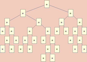
which does, indeed, have 17 leaves.

Quicksort, First Pass

At this point, I can start constructing my purely numeric quicksort function. The basic action of quicksort is to unfold a list into a sorted tree that stores data on its branches before collapsing the tree into a sorted list. At each step, the element in the front of the list is popped off and stored on a tree branch. All the elements in the list which are less than that element are placed in the left branch and all the elements in the list which is greater than that element is stored in the right branch. This makes it a hylomorphism over this kind of tree.

Before getting into the details of the algorithm, we need encodings for all the involved data types. We need basic functions for manipulating;

• Lists
• Lists with a designated minimal and maximal element
• Sorted lists
• Sorted Trees

Since I want everything to be absolutely perfect, I want to bijectively encode all these types, which requires a bit more care.

Lists are the easiest. This will be the initial algebra over X ↦ 1 + ℕ × X. This is a key application for Sierpinski pairing. With Cantor pairing, a random list would tend to have larger elements toward the beginning of the list while Sierpinski pairing will generate random lists with elements closer to the same size. This also means that permutations of the same list will be of more similar size, which won’t hold at all if we used Cantor pairing. I’ll need four combinators to start;

cons[n_, l_] := SierpinskiPair[n, l]+1
head[l_] /; l > 0 := SierpinskiFst[l-1]
tail[l_] /; l > 0 := SierpinskiSnd[l-1]
listFMap[f_] := FinSumMap[1, SierpinskiBimap[#&, f]]

for testing purposes, we can define a few functions to translate back and forth between lists and ℕ.

ListFmap[f_][{0, 0}] := {0, 0}
ListFmap[f_][{1, {n_, m_}}] := {1, {n, f[m]}}

ListUnfoldCoalg[0] := {0, 0}
ListUnfoldCoalg[l_] := {1, {head[l], tail[l]}}
ListUnfold[x_] := ListFmap[ListUnfold][ListUnfoldCoalg[x]]
NatToSList := ListToMList@*ListUnfold

ListFoldAlg[{0, 0}] := 0
ListFoldAlg[{1, {n_, l_}}] := cons[n, l]
ListFold[x_] := ListFoldAlg[ListFmap[ListFold][x]]
SListToNat := ListFold@*MListToList

MListToList comes from my last post. Some tests:

In  := Table[NatToSList[x], {x, 0, 20}]
Out :=
 {{}, {0}, {1}, {0, 0}, {2}, {0, 1}, {1, 0}, {0, 0, 0}, {3},
  {0, 2}, {1, 1}, {0, 0, 1}, {2, 0}, {0, 1, 0}, {1, 0, 0},
  {0, 0, 0, 0}, {4}, {0, 3}, {1, 2}, {0, 0, 2}, {2, 1}}

In  := SListToNat /@ %
Out := {0, 1, 2, 3, 4, 5, 6, 7, 8, 9, 10,
        11, 12, 13, 14, 15, 16, 17, 18, 19, 20}

In  := NatToSList@cons[1, SListToNat@{2, 3, 4}]
Out := {1, 2, 3, 4}

In  := NatToSList@tail[SListToNat@{1, 2, 3, 4}]
Out := {2, 3, 4}

In  := head[SListToNat@{22, 2, 3, 4}]
Out := 22

The other data types are dependent types. This means our operations may vary their behavior depending on a given piece of data which is carried around signifying some structural constraint. The result of a list where all elements are filtered to be more or less than an element will be a list with a structural constraint reflecting that fact. The “fiber” of such a list will be a pair, (m, n), where m is a natural number and n is either a natural number or ∞, the latter signifying no maximal element. We can make functions analogous to those for ordinary lists. The main catch is the situation where the upper limit isn’t ∞. In that case, we’re encoding a list of elements pulled from a finite set, which requires iterating constructors for 1 + n × ℕ instead of 1 + ℕ × ℕ.

boundCons[{b_, ∞}, n_, l_] /; n ≥ b := SierpinskiPair[n - b, l] + 1
boundCons[{b_, t_}, n_, l_] /; b ≤ n ≤ t := in[t - b + 1, n - b][l] + 1

boundHead[{b_, ∞}, l_] /; l > 0 := SierpinskiFst[l - 1] + b
boundHead[{b_, t_}, l_] /; l > 0 := NProj[t - b + 1][l - 1] + b

boundTail[{b_, ∞}, l_] /; l > 0 := SierpinskiSnd[l - 1]
boundTail[{b_, t_}, l_] /; l > 0 := NCodiagonal[t - b + 1][l - 1]

boundListFMap[{b_, ∞}, f_] := FinSumMap[1, SierpinskiBimap[# &, f[{b, ∞}, #]&]]
boundListFMap[{b_, t_}, f_] := FinSumMap[1, FinProdMap[t - b + 1, f[{b, t}, #]&]]

Once these are established, other functions can be defined similarly. We just need to appropriately deliver the fiber to the functions that need it.

BoundListFmap[k_, f_][{0, 0}] := {0, 0}
BoundListFmap[k_, f_][{1, {n_, m_}}] := {1, {n, f[k, m]}}

BoundListUnfoldCoalg[k_, 0] := {0, 0}
BoundListUnfoldCoalg[k_, l_] := {1, {boundHead[k, l], boundTail[k, l]}}
BoundListUnfold[k_, x_] :=
  BoundListFmap[k, BoundListUnfold][BoundListUnfoldCoalg[k, x]]
NatToBoundList[k_, x_] := ListToMList[BoundListUnfold[k, x]]

BoundListFoldAlg[k_, {0, 0}] := 0
BoundListFoldAlg[k_, {1, {n_, l_}}] := boundCons[k, n, l]

BoundListFold[k_, x_] := BoundListFoldAlg[k, BoundListFmap[k, BoundListFold][x]]
BoundListToNat[k_, x_] := BoundListFold[k, MListToList[x]]

Some tests:

In  := Table[NatToBoundList[{0, ∞}, x], {x, 0, 20}]
Out :=
 {{}, {0}, {1}, {0, 0}, {2}, {0, 1}, {1, 0}, {0, 0, 0}, {3},
  {0, 2}, {1, 1}, {0, 0, 1}, {2, 0}, {0, 1, 0}, {1, 0, 0},
  {0, 0, 0, 0}, {4}, {0, 3}, {1, 2}, {0, 0, 2}, {2, 1}}

In  := BoundListToNat[{0, ∞}, #] & /@ %
Out := {0, 1, 2, 3, 4, 5, 6, 7, 8, 9, 10,
        11, 12, 13, 14, 15, 16, 17, 18, 19, 20}

In  := Table[NatToBoundList[{5, 8}, x], {x, 0, 20}]
Out :=
 {{}, {5}, {6}, {7}, {8}, {5, 5}, {6, 5}, {7, 5}, {8, 5}, {5, 6},
  {6, 6}, {7, 6}, {8, 6}, {5, 7}, {6, 7}, {7, 7}, {8, 7}, {5, 8},
  {6, 8}, {7, 8}, {8, 8}}

In  := BoundListToNat[{5, 8}, #] & /@ %
Out := {0, 1, 2, 3, 4, 5, 6, 7, 8, 9, 10,
        11, 12, 13, 14, 15, 16, 17, 18, 19, 20}

In  := NatToBoundList[{0, ∞}, boundCons[{0, ∞}, 1, BoundListToNat[{0, ∞}, {2, 3, 4}]]]
Out := {1, 2, 3, 4}

In  := NatToBoundList[{4, 6}, boundCons[{4, 6}, 5, BoundListToNat[{4, 6}, {4, 5, 6}]]]
Out := {5, 4, 5, 6}

In  := boundHead[{80, ∞}, BoundListToNat[{80, ∞}, {101, 99, 88}]]
Out := 101

In  := NatToBoundList[{80, ∞}, boundTail[{80, ∞}, BoundListToNat[{80, ∞}, {101, 99, 88}]]]
Out := {99, 88}

In  := boundHead[{27, 33}, BoundListToNat[{27, 33}, {30, 31, 32, 33}]]
Out := 30

In  := NatToBoundList[{27, 33}, boundTail[{27, 33}, BoundListToNat[{27, 33}, {30, 31, 32, 33}]]]
Out := {31, 32, 33}

Sorted lists carry around a fiber denoting what the largest element so far is. This guarantees that whatever element is newly added won’t be smaller than the largest element so far. Sorted lists are only more complicated than the last example in the sense that this fiber varies based on the layer of the list (and this is handled entirely by the functorial map); in all other respects sorted lists are simpler.

sortCons[k_, n_, l_] /; n ≥ k := SierpinskiPair[n - k, l] + 1

sortHead[k_, l_] /; l > 0 := SierpinskiFst[l - 1] + k

sortTail[k_, l_] /; l > 0 := SierpinskiSnd[l - 1]

sortListFMap[k_, f_][l_] :=
  FinSumMap[1, SierpinskiBimap[# &, f[sortHead[k, l], #]&]][l]

SortListFmap[k_, f_][{0, 0}] := {0, 0}
SortListFmap[k_, f_][{1, {n_, m_}}] := {1, {n, f[n, m]}}

SortListUnfoldCoalg[k_, 0] := {0, 0}
SortListUnfoldCoalg[k_, l_] := {1, {sortHead[k, l], sortTail[k, l]}}
SortListUnfold[k_, x_] :=
  SortListFmap[k, SortListUnfold][SortListUnfoldCoalg[k, x]]
NatToSortList[k_, x_] := ListToMList[SortListUnfold[k, x]]

SortListFoldAlg[k_, {0, 0}] := 0
SortListFoldAlg[k_, {1, {n_, l_}}] := sortCons[k, n, l]
SortListFold[k_, x_] := SortListFoldAlg[k, SortListFmap[k, SortListFold][x]]
SortListToNat[k_, x_] := SortListFold[k, MListToList[x]]

Some tests:

In  := Table[NatToSortList[0, x], {x, 0, 20}]
Out :=
 {{}, {0}, {1}, {0, 0}, {2}, {0, 1}, {1, 1}, {0, 0, 0}, {3},
  {0, 2}, {1, 2}, {0, 0, 1}, {2, 2}, {0, 1, 1}, {1, 1, 1},
  {0, 0, 0, 0}, {4}, {0, 3}, {1, 3}, {0, 0, 2}, {2, 3}}

In  := SortListToNat[0, #] & /@ %
Out := {0, 1, 2, 3, 4, 5, 6, 7, 8, 9, 10,
        11, 12, 13, 14, 15, 16, 17, 18, 19, 20}

In  := NatToSortList[0, sortCons[0, 1, SortListToNat[1, {2, 3, 4}]]]
Out := {1, 2, 3, 4}

Note that the encoding for {2, 3, 4} has to assume it’s at the end of a list that already had a 1 for the cons to be valid.

In  := sortHead[0, SortListToNat[0, {88, 99, 101}]]
Out := 88

In  := NatToSortList[88, sortTail[0, SortListToNat[0, {88, 99, 101}]]]
Out := {99, 101}

Note that the decoding of the tail has to acknowledge the fact that 88 came before the tail for the decoding to be valid.

Sorted trees were already described in detail in my last post, so I don’t discuss them at length here; I’ll just present my code for them.

sortBranch[{b_, ∞}, n_, t1_, t2_] /; n ≥ b :=
  SierpinskiPair[n - b, CantorPair[t1, t2]] + 1
sortBranch[{b_, t_}, n_, t1_, t2_] /; n ≥ b :=
  in[t - b + 1, n - b][CantorPair[t1, t2]] + 1

sortTreeElem[{b_, ∞}, l_] := SierpinskiFst[l - 1] + b
sortTreeElem[{b_, t_}, l_] := NProj[t - b + 1][l - 1] + b

sortLeft[{b_, ∞}, l_] /; l > 0 := CantorFst[SierpinskiSnd[l - 1]]
sortLeft[{b_, t_}, l_] /; l > 0 := CantorFst[NCodiagonal[t - b + 1][l - 1]]

sortRight[{b_, ∞}, l_] /; l > 0 := CantorSnd[SierpinskiSnd[l - 1]]
sortRight[{b_, t_}, l_] /; l > 0 := CantorSnd[NCodiagonal[t - b + 1][l - 1]]

sortTreeFMap[{b_, ∞}, f_][tr_] := 
  FinSumMap[1,
    SierpinskiBimap[#&, 
      CantorBimap[f[{b, sortTreeElem[{b, ∞}, tr]}, #]&,
                  f[{sortTreeElem[{b, ∞}, tr], ∞}, #]&
  ]]][tr]
sortTreeFMap[{b_, t_}, f_][tr_] :=
  FinSumMap[1, 
    FinProdMap[t-b+1, 
      CantorBimap[f[{b, sortTreeElem[{b, t}, tr]}, #]&,
                  f[{sortTreeElem[{b, t}, tr], t}, #]&
  ]]][tr]

SortTreeFmap[{b_, t_}, f_][L] := L
SortTreeFmap[{b_, t_}, f_][e_[n_, m_]] := e[f[{b, e}, n], f[{e, t}, m]]

SortTreeUnfoldCoalg[k_, 0] := L
SortTreeUnfoldCoalg[k_, l_] := sortTreeElem[k, l][sortLeft[k, l], sortRight[k, l]]
NatToSortTree[k_, x_] := SortTreeFmap[k, NatToSortTree][SortTreeUnfoldCoalg[k, x]]

SortTreeFoldAlg[k_, L] := 0
SortTreeFoldAlg[k_, e_[l_, r_]] := sortBranch[k, e, l, r]
SortTreeToNat[k_, x_] := SortTreeFoldAlg[k, SortTreeFmap[k, SortTreeToNat][x]]

Some tests:

In  := Table[NatToSortTree[{0, ∞}, x], {x, 0, 20}]
Out :=
 {L, 0[L, L], 1[L, L], 0[L, 0[L, L]], 2[L, L], 
  0[0[L, L], L], 1[L, 1[L, L]], 0[L, 1[L, L]], 
  3[L, L], 0[0[L, L], 0[L, L]], 1[0[L, L], L], 
  0[0[L, 0[L, L]], L], 2[L, 2[L, L]], 
  0[L, 0[L, 0[L, L]]], 1[L, 2[L, L]], 
  0[0[L, L], 1[L, L]], 4[L, L], 0[0[L, 0[L, L]],
  0[L, L]], 1[0[L, L], 1[L, L]], 
  0[0[0[L, L], L], L], 2[0[L, L], L]}

In  := SortTreeToNat[{0, ∞}, #] & /@ %
Out := {0, 1, 2, 3, 4, 5, 6, 7, 8, 9, 10,
        11, 12, 13, 14, 15, 16, 17, 18, 19, 20}

In  := Table[NatToSortTree[{5, 9}, x], {x, 0, 20}]
Out :=
 {L, 5[L, L], 6[L, L], 7[L, L], 8[L, L], 9[L, L],
  5[L, 5[L, L]], 6[L, 6[L, L]], 7[L, 7[L, L]], 
  8[L, 8[L, L]], 9[L, 9[L, L]], 5[5[L, L], L], 
  6[5[L, L], L], 7[5[L, L], L], 8[5[L, L], L], 
  9[5[L, L], L], 5[L, 6[L, L]], 6[L, 7[L, L]], 
  7[L, 8[L, L]], 8[L, 9[L, L]], 9[L, 9[L, 9[L, L]]]}

In  := SortTreeToNat[{5, 9}, #] & /@ %
Out := {0, 1, 2, 3, 4, 5, 6, 7, 8, 9, 10,
        11, 12, 13, 14, 15, 16, 17, 18, 19, 20}

With that setup, we can actually start implementing quicksort. There are two recursive algorithms we need beforehand. Firstly, we need a program that takes an element e and a list l with min element b and max element t and returns a pair of lists, the first with min element b and max element e and the second with min element e and max element t. This will be applied each time we want to construct a single layer of our sorted tree.

This algorithm can be implemented as a simple fold. We just recurse over the list, shoving an element into either of the two lists based on its comparison to e (starting with two empty lists) until we run out of elements.

fhylo[fmap_, alg_, coalg_][k_, x_] := 
  alg[k, fmap[k, fhylo[fmap, alg, coalg]][coalg[k, x]]]

bifilterPreAlg[{b_, t_}, e_, h_, lisPair_] :=
  If[h ≤ e,
     CantorBimap[boundCons[{b, e}, h, #]&, #&][lisPair],
     CantorBimap[#&, boundCons[{e, t}, h, #]&][lisPair]
  ]

bifilterAlg[e_][{b_, t_}, l_] /; b ≤ e ≤ t :=
  If[l == 0, 0, 
    bifilterPreAlg[{b, t}, e, boundHead[{b, t}, l], boundTail[{b, t}, l]]
  ]

bifilter[{b_, t_}, e_, l_] := fhylo[{b, t}, boundListFMap, bifilterAlg[e], #2&][l]